Ultrasonic Distance Sensor - 3V or 5V - HC-SR04 compatible - RCWL-1601 & Etape Sensor with Particle Photons
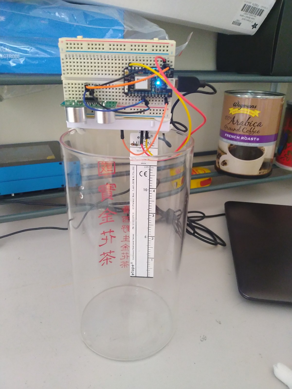
This the sensor we are going to build in this exercise.
This guide is based on these materials:
We will need the following hardwares:
A Particle Photon, it will work with Argon too (Can be bought here)
USB Data Cable
An Ultrasonic Distance Sensor (Can be bought here)
An Etape Sensor (Can be bought here)
Jumper Wires x 4 (Can be bought here)
Breadboard (Can be bought here)
Soldering Kit (Can be bought here)
Laptop or Computer
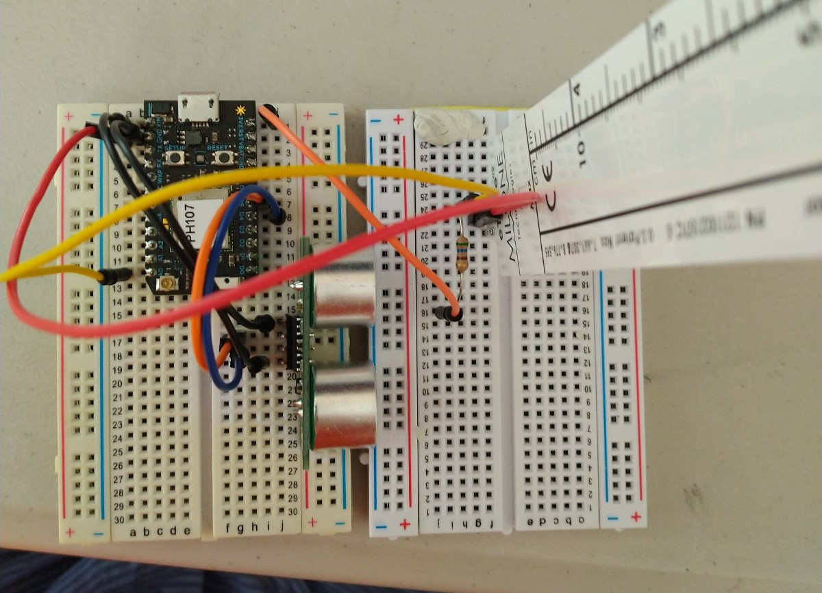
Connect the Photon, Ultrasonic and Etape Sensor onto the breadboard as shown in the figures.
Connect the Ultrasonic sensor as follows
Ultrasonic Sensor <---> Photon
GND <-----------------> GND
VCC <-----------------> VIN
Trig <----------------> D4
Echo <----------------> D5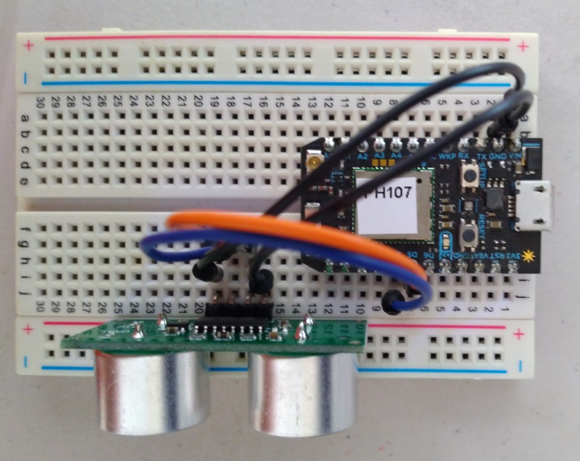
Connect the Etape sensor as follows.
Etape Sensor <---> Photon
Pin 2 -->--<--------> GND
Pin 3 -->-|<--------> A0
    560ohm|
          |<-----> 3V3
The pins diagram of the Etape.

Refer to to register the Photon Device with our Particle account.
Flash the script ‘STAPI_1_RCWL1601_1_ETAPE’ to the Photon. Fill in the mandatory parameters accordingly. You can choose to leave the optional parameters to their default values.
============================================================================================= !!! MANDATORY PARAMETERS ============================================================================================= String thingDesc = "level of water absorbed from the atmosphere for the greenhouse project measured using E-tape and Rangefinder"; //DESCRIBE THE DEPLOYMENT int sample_rate = 5 * 1000; // how often you want device to publish where the number in front of a thousand is the seconds you want ============================================================================================= OPTIONAL PARAMETERS (this parameters only works when it is the first time registration of the device) (if the device is already registered, these options are ignored) ============================================================================================= // the value of the 'other' resistor #define SERIESRESISTOR 560 // What pin to connect the sensor to #define SENSORPIN A0 int trigPin = D4; int echoPin = D5; //Description of the location String foiName = "na"; //THE LOCATION NAME String foiDesc = "na"; //Define the geometry of the location. Geometry types from geojson is accepted. Refer to https://tools.ietf.org/html/rfc7946 for geometry types. String locType = "Point"; String enType = "application/vnd.geo+json"; //Define the location of the thing. If location is not impt, use [0,0,0] the null island position. float coordx = 0.0; //lon/x float coordy = 0.0; //lat/y float coordz = 0.0; //elv/zIt is advised to calibrate the Etape sensor. This is the Python script used to the length of the tape with the associated resistance read from the sensor. The script requires you to pour the right level of water and measure the corresponding resistance. A linear relationship is then established between the resistance measured and the length on the tape.
import psycopg2
from sshtunnel import SSHTunnelForwarder

import matplotlib.pyplot as plt
import numpy as np

def get_data_frm_db(st_time, end_time, ds_id, cursor):
    ds_id = str(ds_id)
    command =   """
                SELECT "RESULT_NUMBER"
                FROM public."OBSERVATIONS"
                WHERE "DATASTREAM_ID" = %s and "RESULT_TIME" > '%s' and "RESULT_TIME" < '%s';
                """ %(ds_id, st_time, end_time)

    cursor.execute(command)
    rows = cursor.fetchall()
    return rows

def avg_data(st_time, end_time, ds_id, cursor):
    datas = get_data_frm_db(st_time, end_time, ds_id, cursor)
    ndata = float(len(datas))
    totald = 0
    for d in datas:
        totald = totald + d[0]
    avg = totald/float(ndata)
    return avg

#==========================================================================================
#MAIN SCRIPT
#==========================================================================================
xls = []
yls = []

PORT=5432
with SSHTunnelForwarder(('andlchaos300l.princeton.edu'),
                        ssh_username='',
                        ssh_password='',
                        remote_bind_address=('localhost', PORT),
                        local_bind_address=('localhost', PORT)):

    try:
        conn = psycopg2.connect(dbname='spatempdb',
                                user='',
                                host='localhost',
                                port = 5432,
                                password='')
        cursor = conn.cursor()
        print('connected', cursor)
    except:
        print('notconnected')

    ds_id = 95
    st_times = [['2021-08-13 19:15:00-4', '2021-08-13 20:00:00-4'],#1 inch
                ['2021-08-13 20:02:00-4', '2021-08-13 20:50:00-4'],#1.5
                ['2021-08-13 20:55:00-4', '2021-08-13 21:50:00-4'],#2
                ['2021-08-13 21:56:50-4', '2021-08-13 22:05:00-4'],#2.5
                ['2021-08-13 22:19:00-4', '2021-08-13 23:25:00-4'],#3
                ['2021-08-13 23:45:00-4', '2021-08-14 00:10:00-4'],#3.5
                ['2021-08-14 00:20:00-4', '2021-08-14 00:40:00-4'],]#4
                #['2021-08-14 00:50:00-4', '2021-08-14 01:02:00-4']]#4.5

    lengths = [1, 1.5, 2, 2.5, 3, 3.5, 4, 4.5]
    for cnt, time_range in enumerate(st_times):
        st_time = time_range[0]
        end_time = time_range[1]
        # # using all the data to construct the curve
        # res_list = get_data_frm_db(st_time, end_time, ds_id, cursor)
        # for res in res_list:
        #     xls.append(res[0])
        #     yls.append(lengths[cnt])

        # using only the averages to construct the curve
        avg_res = avg_data(st_time, end_time, ds_id, cursor)
        xls.append(avg_res)
        yls.append(lengths[cnt])

    cursor.close()

xls = np.array(xls)
xls = xls.reshape([-1,1])

yls = np.array(yls)
yls = yls.reshape([-1,1])

print(xls)
#===========================================================================================
#POLYNOMIAL CURVE FITTING
#===========================================================================================
from sklearn.linear_model import Ridge
from sklearn.preprocessing import PolynomialFeatures
from sklearn.pipeline import make_pipeline

colors = ['teal', 'yellowgreen', 'gold']
lw = 2

for count, degree in enumerate([1]):
    model = make_pipeline(PolynomialFeatures(degree), Ridge())
    model.fit(xls, yls)
    ypred = model.predict(xls)
    ridge = model.named_steps['ridge']
    coef = ridge.coef_[0]
    intercept = ridge.intercept_[0]
    # 1 degree y = mx + c
    # 2 degree curve (y = ax^2 + bx + c)
    # 3 degree curve (y = ax^3 + bx^2 + cx + d )

    print(coef, intercept)
    ypred2s = []
    for i in range(len(xls)):
        # ypred2 = coef[1]*xls[i][0]**1 + coef[2]*xls[i][0]**2 + coef[3]*xls[i][0]**3 + intercept
        ypred2 = coef[1] * xls[i][0] + intercept
        ypred2s.append(ypred2)

    # print(ypred2s)
    # print(ypred)

    plt.plot(xls, ypred, color=colors[count], linewidth=lw,
             label="degree %d" % degree)

# Plot outputs
plt.scatter(xls, yls, color='black')
# plt.plot(xls, ypred, color='blue', linewidth=3)
plt.show()